The 3DMatch program is developed for pair alignment of proteins 3D-structures.
The input data for the program are PDB files of two structures and chains' identifiers.
The output data - PDB file that contains atomic coordinates for optimally aligned
3D-structures of proteins. Moreover, in the PDB file in the field "REMARK 1" values for
RMSD and Zscore are represented. As well in this field the pair alignment of sequences,
built on the basis of structural alignment, and its characteristics, including the number
of aligned positions, gaps and aminoacid matches (in percents), is represented.
Comparing 3DMatch and CE
To compare alignments performed by 3DMatch and widely distributed program CE it was compiled a set of 490 protein pairs. Pairs were compiled by the random selection of proteins with common structural domains from the SCOP database. Each protein pair was aligned with use of 3DMatch and CE. On the output, alignments performed by CE were found to have the RMSD values for all pairs lower in average for 0.13 angstroms than those performed by 3DMatch. The number of aligned positions obtained with use of 3DMatch, however, was higher in average for 5.03 than those for CE. In some cases, the length of 3DMatch performed alignment exceeded the CE performed one for more then 100 residues.
Some examples of 3DMatch and CE comparing:
| PDB Id | RMSD 3DMatch/CE | Aligned positions 3DMatch/CE |
| 1DAR:_ - 1FNM:A | 2.3/0.8 | 604/451 |
| 1FFY:A - 1IVS:A | 3.7/3.3 | 732/604 |
| 1LT3:A - 1XDT:T | 3.7/7.0 | 102/72 |
| 1EZX:C - 1DLE:A | 2.4/2.9 | 140/96 |
Algorithm Description
Algorithm for structural aligning realizes two approaches: The approach based on aligning the secondary structure elements (SSE), and the one based on aligning by Ca atoms. As a result, two specific for each approach alignments are created, and the program, using the Zscore criterion, chooses the best one for the output.
Each of two approaches uses 3-step process for aligning protein three-dimensional structures, including the search for alignment core with the best RMSD, its expansion by adding new fragments of protein to the alignment, and optimization with use of dynamic programming to achieve an optimal alignment.
1. Algorithm of Structural Aligning by Secondary Structure Elements.
Calculation of coordinates for protein secondary structure elements.
Using C, Ca and N atomic coordinates, the secondary structure is calculated. The secondary structure is represented by two types of elements: alpha-helix and beta-folds. Using the Ca atomic coordinates, the coordinates for geometric centre of mass are calculated for each SSE. Thus, the protein's 3D-Structure is defined by coordinates for SSE's centers of mass. Transition from atomic coordinates for each residue to the coordinates for SSE's centers of mass allows to significantly decrease the number of dimensional points that describe the protein 3D structure.
Building the core of alignment.
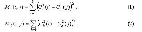
Two structures, for which the pair structural alignment should be built, are being analyzed. For each structure the matrix of pair distances between SSE is being calculated, M1 for the first structure and M2 for the second one:
where i, j are indices for SSE, C1k defines x, y, z coordinates for SSE. For matrix M1, i, j = 1, N1, for M2, i, j = 1, N2, where N1 is a number of SSE for protein 1, N2 is the same for protein 2.
Further the overhaul of combinations for SSE pairs composed from SSE of first and second proteins is being performed. Pairs are formed only for SSE that belongs to the same type of secondary structures, i.e. the pair must consist of SSE of the same type. Each pair is considered as starting point for further aligning.
Let the starting point is the pair SSE1i and SSE2j, where i is the index for SSE in the first structure and j is the index for SSE in the second structure. Further task is to find such two ensembles P={SSE1i, SSE 1i+k1, SSE 1i+k2, …, SSE 1i+kn.}, where 0<k1<k2 … < kn and Q={SSE2j, SSE2j+m1, SSE2j+m2, ..., SSE2j+mn}, where 0<m1<m2 … < mn, so that RMSD(P,Q) would not exceeded the threshold value when n is maximal. Composing of ensembles P and Q, which determine the way of alignment, is based on "quickest descend" approach. The sequential adjunction of elements of these ensembles is being performed. At every step the overhaul of possible variants is performed. Among these variants the only one with the lowest RMSD is selected, at this the RMSD value must be lower than threshold one. Let ensembles P and Q contain q elements and it is required to add a q+1 element. Let P(q+1) = SSE1k, Q(q+1) = SSE2m. Then RMSD for q+1 element of Q1 and Q2 ensembles is calculated by the following way:
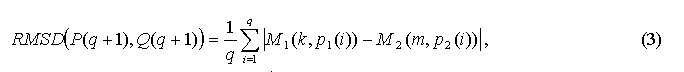
where p1(i) and p2(i) are the indices for ith SSE of ensembles P and Q, respectively.
Thus, for every starting point of alignment, the ensembles P and Q are being composed, and among them the one (P,Q) with maximal length is selected. Evaluation of structural similarity of two proteins based on the described algorithm, that does not include conversion of coordinates and calculation of turns and shifts, possesses a significant processing speed. This evaluation is, however, very approximate and since the further sorting of pairs (P,Q) with similar length is performed by direct superposition of two ordered ensembles of points from . For superposed structures the RMSD is calculated as Euclidean distance in the space between superposing points
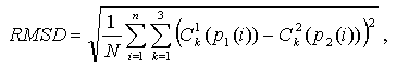
where N is the length of ensembles P,Q.
When the lengths of alignments are the same, an alignment with the lowest RMSD is selected.
The best superposition of two structures
The task of superposing two ordered ensembles P={P1,P2,...,PN} and Q={Q1,Q2,...,QN} of points from R3 is focused on determination of rigid-body conversion (x0, T): R3—>R3 , that provides the minimal value for functional:
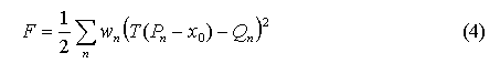
under condition
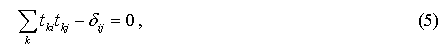
where x0 - the shift vector, T=(tij) - rotation matrix, dij - elements of the unitary matrix. To determine the rotation matrix, it was used the approach based on direct solution of task for minimization of current functional (Kabsch, 1976)
To solve this task, it is introduced a symmetric matrix of Lagrange multipliers L=(lij), that is used to define a supplementary function:
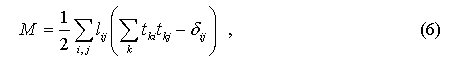
that is added to F to form Lagrangian function:
![]()
To find the minimum of F with restrictions (5), it is necessary to determine the minimum of functional (7). To solve this task, the matrix R=(rij) is being built
![]()
Preliminarily, the shift problem is being avoided by replacing the system of coordinates of each set of points to their centre of mass. For matrix that is product of RTR , where RT is the transposed matrix R , the eigenvalues mk and corresponding to them eigenvectors, that form matrix ak, are being determined. Further the values of bk matrix are calculated by the following formula:
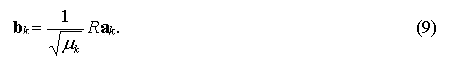
Values of target matrix T are calculated as product of elements of matrices bk and akT
![]()
If one of eigenvalues of the matrix RTR is equal to zero, for example m3 =0, the corresponding columns of matrices ak and bk are being built by other two columns:
![]()
Transformation of alignment by SSE into alignment by Ńa atoms
On the next step of algorithm, when the core of alignment for SSE is built, it is being transformed into alignment by Ńŕ atoms. At this moment we have two dimensionally superposed protein structures and superposing was performed by coordinates of center of mass of SSEs. For switch to superposing by Ca atoms the global dynamic programming with use of Needleman-Wunsch algorithm is applied. Superposing by SSE is used as an initial dimensional location of molecules, which further will be corrected with use of dynamic programming.
In a protein sequence a continuous fragment, starting and ending positions of which are determined by the first and last SSE in ensembles P for the first protein and Q for the second one, is selected. Matrix of proximity between residues of two fragments is being built in accordance to the rule:
Dij=Con-dij
Con is a constant, dij is Euclidean distance between ith č jth Ńŕ atoms atoms, taken from the first and the second structures respectively. After the global aligning is performed with use of dynamic programming, we have a pair alignment for fragments' sequences. Further, in accordance with obtained alignment, a dimensional superposing of structures, i.e. switching from an aligning by sequence to a structural one, is being performed. To achieve this, the previously described algorithm of the best superposition of two structures is used.
Expansion of alignment core
The next step of algorithm is an expansion of the alignment core that results in extending of N- and C-ends of sequence's fragment included in alignment. Search for new location of starting and ending positions of alignment fragment in a sequence is performed. The search is performed by scanning the frame of a certain length. RMSD values for Ca atoms between the frame sliding along the first and the second sequences are calculated. As new N- and C-ends the outermost frame locations, providing the RMSD lower than threshold, are used. Further, for extended fragments of the first and the second sequences, the Dij matrix is calculated and dynamic programming is applied to it to obtain new alignment.
Optimization of the alignment
Optimization of the alignment is performed with use of cyclic reference to dynamic programming that results in calculation of alignment by sequence and then its conversion into structural one. Such a process is being repeated multiple times with little variations for gap penalties. As a resulting alignment the one with lowest RMSD and biggest length is accepted.
2. Algorithm for structural alignment by Ca atoms.
This algorithm does not use the information on a protein secondary structure. The algorithm is analogous to that for alignment by SSE with a single exception: instead of SSE the fragments of sequence with length of 8 residues are used. There is one more difference: SSE are not-overlapping regions of sequence, while in this algorithm the fragments overlap each other with shift for 1 residue. In performance the algorithm for alignment by Ca atoms significantly yields to that for alignment by SSE. Moreover, during the building of alignment core it is more susceptible to local minimums that results in missing the real alignment. It, however, possesses a number of advantages. First of all, the algorithm for alignment by Ńŕ atoms atoms can work for proteins that lack secondary structure, i.e. do not contain helixes or beta-folds and are represented by loops only. Moreover, the presence in protein of very large loops may result in lowering of quality for alignment by SSE, while alignment by Ńŕ atoms atoms is invariant to secondary structure type. It should also be noted that this algorithm does not depend on quality of secondary structure recovery by atomic coordinates, while for alignment by SSE it is critical.
Output data
Structural alignment is being represented in PDB format, in which the queried structures are given different chain IDs. In the REMARK field the values for Root Mean Square Deviation (RMSD), Zscore and structure-based sequence alignment are being put.
Zscore is a measure of the statistical significance of structural alignment of queried proteins relative to an alignment of random structures. Typically proteins with a similar fold will have a Zscore of 3.5 or better.
Example of output data:
HEADER    PROTEIN STRUCTURE ALIGNMENT
COMPND    (A) 1BWW chain A (B) 2BFV chain L
REMARK   1
REMARK   1 RMSD on Ca-atoms :  0.817 angstrom
REMARK   1 Zscore           :  6.230
REMARK   1 Aligned positions:    107
REMARK   1 Gap positions    :      5
REMARK   1 Sequence identity:   54.5 (%)
REMARK   1
REMARK   1 Structure based sequence alignment
REMARK   1
REMARK   1 3     DIQMTQSPSSLSASVGDRVTITCQASQDII-----KYLNWYQQKPGKAPKLLIYEASNLQ
REMARK   1 1     DIELTQSPPSLPVSLGDQVSISCRSSQSLVSNNRRNYLHWYLQKPGQSPKLVIYKVSNRF
REMARK   1
REMARK   1 58    AGVPSRFSGSGSGTDYTFTISSLQPEDIATYYCQQYQSLPYTFGQGTKLQIT
REMARK   1 61    SGVPDRFSGSGSGTDFTLKISRVAAEDLGLYFCSQSSHVPLTFGSGTKLEIK
REMARK   1
ATOM      1  N   THR A   1     -19.249   5.700 -17.692  1.00 67.85           N
ATOM      2  CA  THR A   1     -18.745   6.056 -16.364  1.00 64.75           C
ATOM      3  C   THR A   1     -17.224   6.135 -16.364  1.00 48.48           C
ATOM      4  O   THR A   1     -16.538   5.185 -16.770  1.00 47.02           O
ATOM      5  CB  THR A   1     -19.208   5.088 -15.261  1.00 72.33           C
ATOM      6  OG1 THR A   1     -20.156   4.118 -15.725  1.00 76.14           O
ATOM      7  CG2 THR A   1     -19.920   5.864 -14.157  1.00 80.20           C
ATOM      8  N   PRO A   2     -16.625   7.231 -15.917  1.00 34.29           N
ATOM      9  CA  PRO A   2     -15.148   7.268 -15.925  1.00 29.06           C
ATOM     10  C   PRO A   2     -14.623   6.268 -14.892  1.00 29.14           C
ATOM     11  O   PRO A   2     -15.235   6.026 -13.852  1.00 27.39           O
ATOM     12  CB  PRO A   2     -14.808   8.683 -15.482  1.00 28.31           C
ATOM     13  CG  PRO A   2     -16.083   9.426 -15.367  1.00 30.57           C
ATOM     14  CD  PRO A   2     -17.184   8.412 -15.270  1.00 32.32           C
ATOM     15  N   ASP A   3     -13.462   5.687 -15.144  1.00 27.28           N
ATOM     16  CA  ASP A   3     -12.894   4.816 -14.115  1.00 21.41           C