alon1999

Content

1. Introduction
2. Running the application and loading data.
3. Hierarchical clustering of experiments.
4. References

1. Introduction

Using SelTag software the alon1999_set.txt data were analyzed. The data contain measurements of expression levels of 2000 human cDNAs and ESTs (including sequences homologous to some known eukaryotic genes) in colon adenocarcinoma tissues from several patients. For some patients, expression of these RNAs was also measured in normal colon tissues. Totally the table contains the measurements of expression in 40 tumor and 22 normal colon tissues. These data are combined into appropriate measurement groups "Tumor" and "Normal". Analysis consisted in building the hierarchical clustering for tissues. It was obtained the division of tissues (experiments) into two classes. The first class includes predominantly tumor tissues, the second one - normal. Results were compared to the ones obtained in original paper [1].

2. Running the application and loading data.

2.1. On the application startup the "Login" dialog window appears (fig. 2.1). In this window select the "Anonymous" mode and press the "OK" button.
Note. The "Anonymous" mode is intended for working with demo data.

Figure 2.1.

1. Non-registered user mode. 2. Button to run application. 3. Button to cancel the application start.

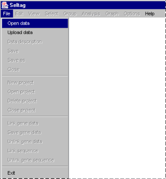
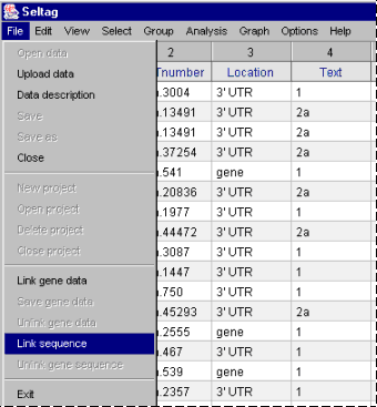
2.2. After the application is started the main application window appears. Select the "File>Open data" command in the main menu (fig. 2.2)

Figure 2.2.

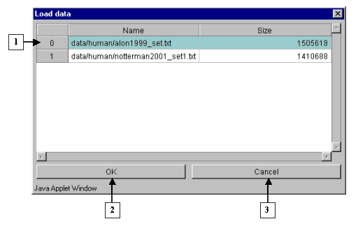
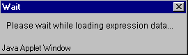
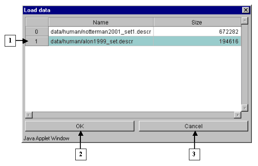
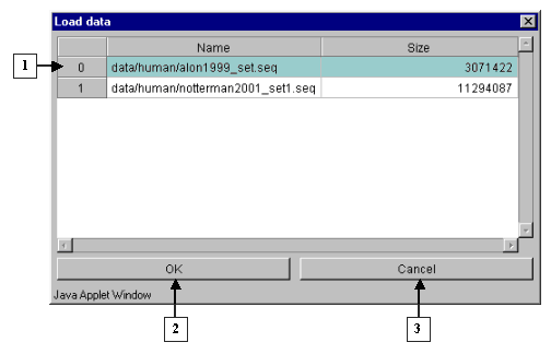
2.3. Once it is done, appears the "Load data" dialog window that contains the names of files with data tables and sizes of these files (fig. 2.3.1). In this window select a file and press the "OK" button. It will cause appearance of the "Wait" message box, which will disappear after finishing of data loading (fig. 2.3.2).

Figure 2.3.1.

1. Selected file with expression data. 2. Confirmation button. 3. Cancel button.

Figure 2.3.2.

2.4. Table with the selected data will be shown in the main application window.

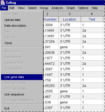
2.5. To load a file with genes description select the "File>Link gene data" command in the main menu (fig. 2.5).

Figure 2.5.

2.6. The "Load data" dialog window that contains the names of files with genes descriptions and sizes of these files will appear (fig. 2.6). In this window select a file and press the "OK" button.

Figure 2.6.

1. Selected file with genes description. 2. Confirmation button. 3. Cancel button.

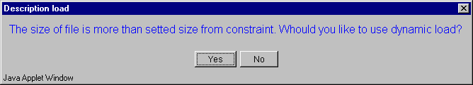
2.7. The "Description load" message box with suggestion to use dynamic file loading mode (fig. 2.7) will appear. Press the "Yes" button.

Figure 2.7.

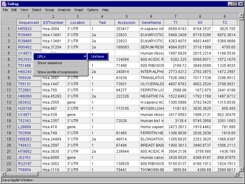
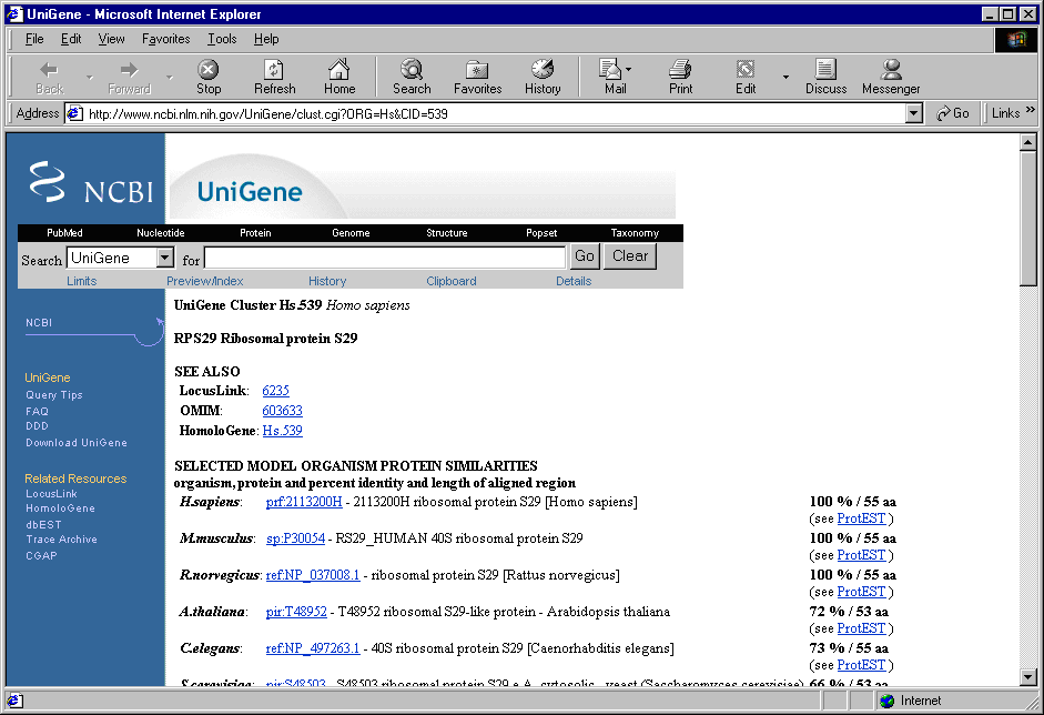
2.8. In contextual menu of the application main table (contextual menu can be called out by the right mouse click) the "URLs>UniGene" command will become active (fig. 2.8.1). This command, using a web link to gene, loads a card from UniGene database for the appropriate gene into new window of your web browser (fig. 2.8.2).

Figure 2.8.1.

Figure 2.8.2.

2.9. To load a file with gene's nucleotide sequences, select the "File>Link sequence" command in the main menu (fig. 2.9).

Figure 2.9.

2.10. It will result in appearance of the "Load data" dialog window that contains the names of files with genes' sequences and information on sizes of these files (fig. 2.10). In this window select a file and press the "OK" button.

Figure 2.10.

1. Selected file with genes description. 2. Confirmation button. 3. Cancel button.

2.11. Further the "Description load" message box with suggestion to use dynamic file loading mode (fig. 2.11) will appear. Press the "Yes" button.

Figure 2.11.

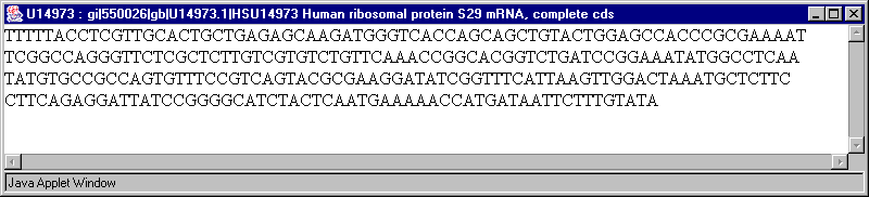
2.12. In contextual menu of the application main table (contextual menu can be called out by the right mouse click) the "Show sequence" command will become active (fig. 2.8.1). This command calls out the window with nucleotide sequence of a gene (fig. 2.12).

Figure 2.12.

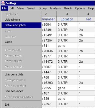
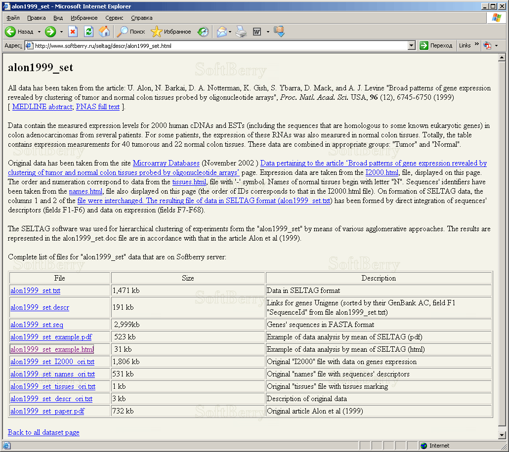
2.13. To retrieve a description of loaded data, select the "File>Data description" command in the main menu (fig. 2.13).

Figure 2.13.

2.14. It will result in opening of a document with description and list of files for data "alon1999_set" from the Softberry server (fig. 2.14).

Figure 2.14.

3. Hierarchical clustering of experiments.

One of the approaches for revealing clusters of genes with similar profiles of expression is the method of hierarchical clustering [2]. Such an analysis is based on building of binary tree for experiments by defined metrics of distances between them. Each knot of a tree connects two child knots, lengths of branches correspond to distances between expression profiles in experiments.

This chapter contains description of the building of trees for fields with use of various methods of hierarchical clustering as well as comparison of obtained clustering results with original ones [1].

To perform the claimed task it is necessary to do the following:

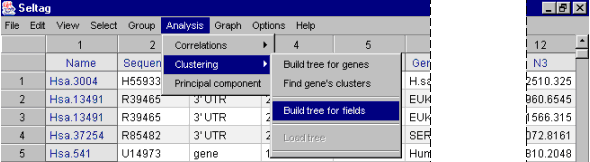
3.1. Select the "Clustering>Build tree for fields" command in the main menu (fig. 3.1).

Figure 3.1.

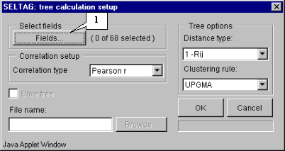
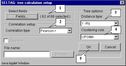
3.2. It will cause opening of the "Tree calculation setup" dialog (fig. 3.2). For the beginning, choose fields that will be used for calculation. To do this press the "Fields" button (fig. 3.2).

Figure 3.2.

1. Button for opening of the "Field selection" dialog window.

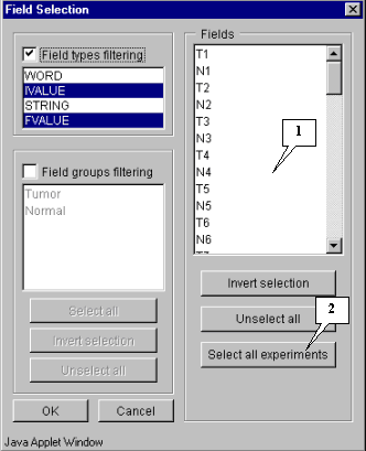
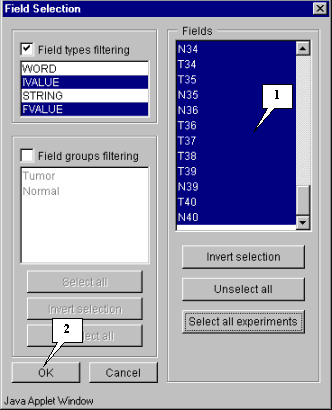
3.3. The "Field selection" dialog (fig. 3.3) that is purposed for fields selection will appear. In the current example, all experiments are involved in calculation. Press the "Select all experiments" button.

Figure 3.3.

1. Fields selection list. 2. Button for selecting of all fields with data on experiments.

3.4. It will result in selecting of all fields that contain expression values (fig. 3.4). Press the "OK" button.

Figure 3.4.

1. Selected fields with data on experiments. 2. Confirmation button.

3.5. In the "Tree calculation setup" dialog, alongside to the "Fields" button, the information on number of selected fields will appear (fig. 3.5).

Figure 3.5.

1. Information on number of selected fields. 2. List of correlation types. 3. List of distance types. 4. List of clustering rules. 5. Confirmation button.

3.6. Further actions are required:

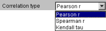
3.6.1. To choose the appropriate variant from the "Correlation type" list (fig. 3.6.1.).

Figure 3.6.1.

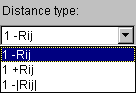
3.6.2. To choose the type of distances (that are calculated in dependence on correlation coefficient Rij) from the "Distance type" list (fig. 3.6.2.).

Figure 3.6.2.

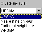
3.6.3. To choose the clustering method from the "Amalgamation rule" list (fig. 3.6.3.).

Figure 3.6.3.

3.6.4. To press the "OK" button.
Example of settings is shown on fig. 3.5.

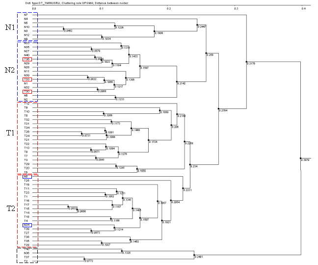
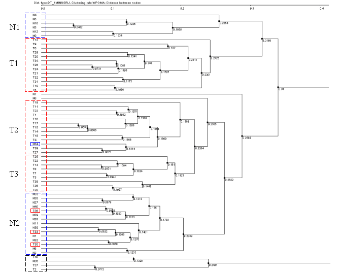
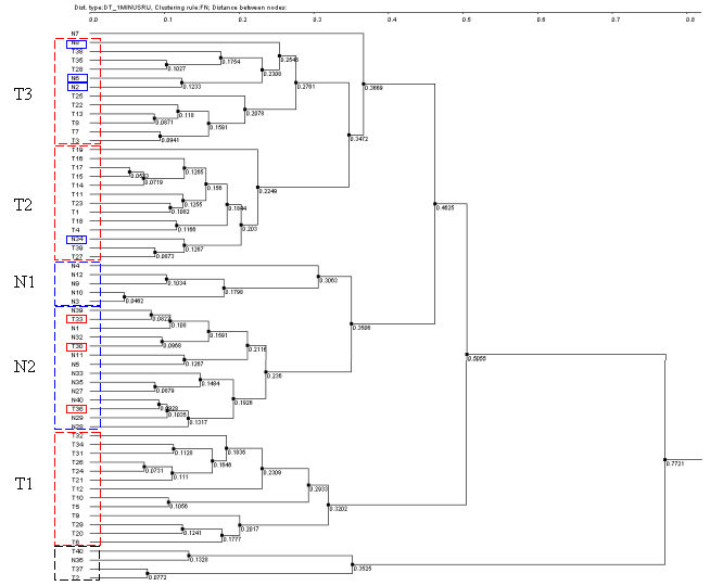
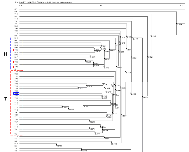
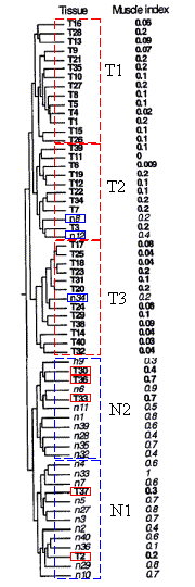
3.7. It will cause the "Tree Diagram" dialog with obtained fields tree diagram to appear. On figures 3.7-3.10 the diagrams obtained with use of different knot binding ways are shown. To build the diagrams the following parameters shown on fig. 3.5 (Pearson's correlation and 1-Rij type of distance) were used. The figure 3.7 represents the results of using the UPGMA knots binding way, the fig. 3.8 - the WPGMA one, the fig 3.9 - the Furthest neighbor type, and the fig 3.10 - the Nearest neighbor one.

Figure 3.7.

Figure 3.8.

Figure 3.9.

Figure 3.10.

On all diagrams shown the tissues are clearly divided into cancerous and normal ones, and for all diagrams the clusters of normal tissues contain the cancerous tissues T30, T33 and T36, while the clusters of cancerous tissues include the normal ones N34 (for all 4 diagrams) and N8 (for those built with use of Furthest neighbor and UPGMA types) that is in accordance to results obtained by Alon et al., 1999. Three diagrams (UPGMA, WPGMA and Furthest neighbor) contain a small cluster of N36, T2, T37 and T40 tissues that is stably being excluded from common pull.

The first cluster of normal tissues (N1) contains the common for all methods tissues N3, N4, N9, N10 and N12. In the article for this cluster described N3, N4, and N10 ones.
The second cluster of normal tissues (N2) contains the common for all methods tissues N1, N11, N27, N28, N29, N32, N33, N35, N39, and N40 as well as previously mentioned T30, T33 and T36. In the article for this cluster described N1, N11, N28, N32, N35, N39 and T30, T33 and T36 ones.
The cluster of cancerous tissues T1 contains the common for all three methods tissues T5, T6, T9, T10, T12, T20, T21, T24, T26, T29, T31, T32 and T34, and content of this cluster is identical for WPGMA and Furthest neighbor methods.
The cluster of cancerous tissues T2 contains the common for all three methods tissues N34, T1, T4, T11, T14, T15, T16, T17, T18, T19, T23, T27 and T39, and content of this cluster is identical for WPGMA and Furthest neighbor methods.
The cluster of cancerous tissues T3 contains the common for WPGMA and Furthest neighbor methods tissues T3, T7, T8, T13, T22, T25, T28, T35 and T38.

Thus, the analysis of clusters content by the methods described shows the stability of data clustering process.

Table 1. Content of clusters for methods UPGMA and Furthest neighbor (FN), and for results described in the article. In the "original" columns the order of cluster fields corresponding to tree is shown, the "sort" one contains the fields sorted by numbers. Clusters enumeration corresponds to that on figures 3.8-3.10. The numbers for normal tissues that are included in cancerous cluster, as well as that for cancerous ones that are included in normal cluster, are shown in red.

Cluster name	Paper		UPGMA		FN		WPGMA
Cluster name	original	sort	original	sort	original	sort	original	sort
T1	T16	T1	T12	T3	T32	T5	T12	T5
	T28	T4	T9	T5	T34	T6	T9	T6
	T13	T5	T10	T6	T31	T9	T6	T9
	T9	T8	T5	T7	T26	T10	T29	T10
	T21	T9	T32	T8	T24	T12	T20	T12
	T35	T10	T31	T9	T21	T20	T34	T20
	T10	T13	T34	T10	T12	T21	T26	T21
	T27	T15	T26	T12	T10	T24	T24	T24
	T8	T16	T24	T13	T5	T26	T21	T26
	T5	T21	T21	T20	T9	T29	T32	T29
	T4	T26	T22	T21	T29	T31	T31	T31
	T1	T27	T13	T22	T20	T32	T10	T32
	T15	T28	T8	T24	T6	T34	T5	T34
	T26	T35	T7	T26
			T3	T29
			T29	T31
			T20	T32
			T6	T34

T2	T17	N34	N8	N8	T19	N34	T19	N34
	T25	T14	T25	N34	T15	T1	T11	T1
	T18	T17	T19	T1	T17	T4	T23	T4
	T23	T18	T11	T4	T16	T11	T1	T11
	T31	T20	T23	T11	T14	T14	T16	T14
	T20	T23	T1	T14	T11	T15	T17	T15
	N34	T24	T16	T15	T23	T16	T15	T16
	T24	T25	T17	T16	T1	T17	T14	T17
	T29	T29	T15	T17	T18	T18	T18	T18
	T38	T31	T14	T18	T4	T19	T4	T19
	T14	T32	T18	T19	N34	T23	N34	T23
	T40	T38	T4	T23	T39	T27	T39	T27
	T32	T40	N34	T25	T27	T39	T27	T39
			T39	T27
			T27	T28
			T38	T35
			T35	T38
			T28	T39

T3	T39	N8			N8	N2	T25	T3
	T11	N12			T38	N6	T22	T7
	T6	T3			T35	N8	T13	T8
	T19	T6			T28	T3	T8	T13
	T12	T7			N6	T7	T7	T22
	T22	T11			N2	T8	T3	T25
	T34	T12			T25	T13	T38	T28
	T7	T19			T22	T22	T35	T35
	N8	T22			T13	T25	T28	T38
	T3	T34			T8	T28
	N12	T39			T7	T35
					T3	T38

N1	N4	N2	N7	N3	N4	N3	N4	N3
	N33	N3	N4	N4	N12	N4	N5	N4
	N7	N4	N5	N5	N9	N9	N10	N5
	T37	N5	N10	N7	N10	N10	N3	N9
	N5	N7	N3	N9	N3	N12	N12	N10
	N27	N10	N12	N10			N9	N12
	N3	N27	N9	N12
	N2	N29
	N40	N33
	N36	N36
	T2	N40
	N29	T2
	N10	T37

N2	N9	N1	N33	N1	N39	N1	N33	N1
	T30	N6	N35	N2	T33	N5	N35	N2
	T36	N9	N27	N6	N1	N11	N27	N6
	N6	N11	N40	N11	N32	N27	N40	N11
	T33	N28	T36	N27	T30	N28	T36	N27
	N11	N32	N29	N28	N11	N29	N29	N28
	N1	N35	N28	N29	N5	N32	N28	N29
	N39	N39	N11	N32	N33	N33	N11	N32
	N28	T30	N39	N33	N35	N35	N39	N33
	N35	T33	T33	N35	N27	N39	T33	N35
	N32	T36	N1	N39	N40	N40	N1	N39
			N32	N40	T36	T30	N32	N40
			T30	T30	N29	T33	T30	T30
			N6	T33	N28	T36	N6	T33
			N2	T36			N2	T36

Figure 3.1.1.

4. References

1. Alon U, Barkai N, Notterman DA, Gish K, Ybarra S, Mack D, and Levine AJ (1999) Broad patterns of gene expression revealed by clustering of tumor and normal colon tissues probed by oligonucleotide arrays, Proc. Natl. Acad. Sci. USA, 96, 6745-6750.

2. Sneath P.H.A., Sokal R.R. (1973) Numerical Taxonomy. The principles and practice of numerical classification. San Francisco: W.H. Freeman and Co.