Figure 2.1.
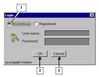
1. Anonymous (non registered user) mode.
2. Confirmation button.
3. Cancel button.
Using the "SelTag" software the data on gene expression from the "notterman2001_set1.txt" file were analyzed. The data consist of measured expression levels for approximately 7400 human cDNAs and ESTs (Human 6500 GeneChip Set, Affymetrix) in colon adenocarcinomas from several patients (Notterman et al., 2001). Expression levels were also measured in normal colon tissues. Totally the table contains the expression measurements for 18 tumor and 18 normal counterpart colon tissues. These data are divided into "Tumor" and "Normal" groups. Data in columns of expression matrix were normalized in such a way that average value was equal to 50. The aims of analysis were the following:
2.1.
On the application startup the "Login" dialog window appears (fig. 2.1). In this window select the "Anonymous" mode and press the "OK" button.
Note. The "Anonymous" mode is intended for working with demo data.
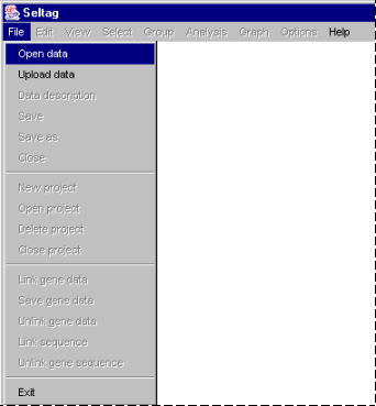
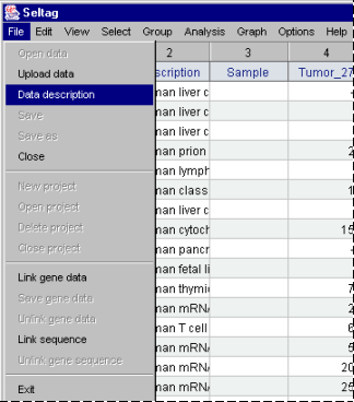
2.2. Once the login procedure is over, the application main window appears. To load data from file, select the "File>Open data" command from the main menu (fig. 2.2).
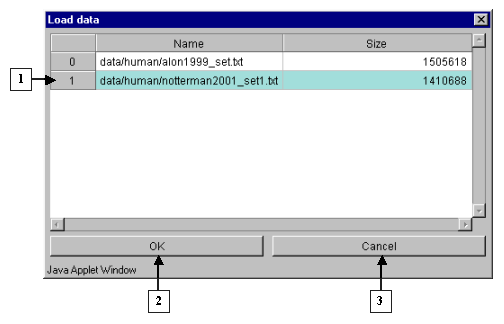
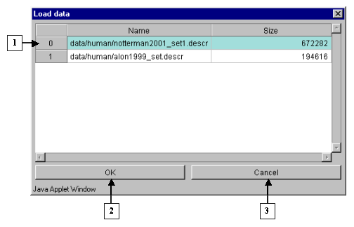
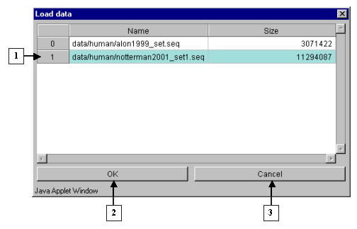
2.3. It will cause the "Load data" window, containing the names of files with table data and information on their size (fig. 2.3.1), to appear. Choose the appropriate filename and press "OK". The "Wait" message window will appear indicating the data loading process, and once the process is over, it will disappear (fig. 2.3.2)
2.4. Table with selected data will be represented in the application main window.
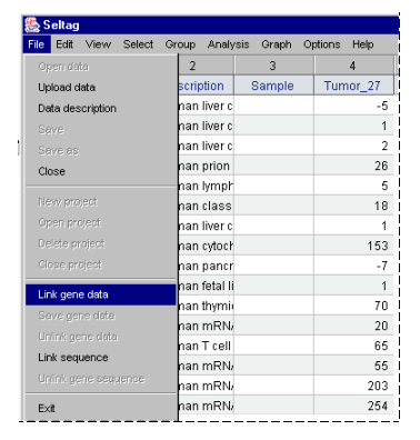
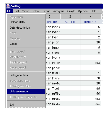
2.5. To load a file with genes description, select the "File>Link gene data" command from the main menu (fig. 2.5).
2.6. The "Load data" dialog with list of files and information on their size (fig. 2.6) will appear. Choose the file of interest and press "OK".
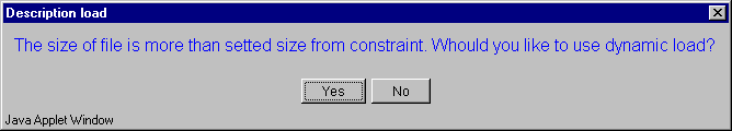
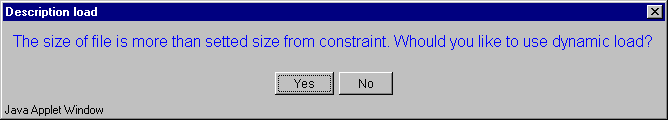
2.7. The "Description load" dialog with invitation to use dynamic file loading mode (fig. 2.7) will appear. Press the "Yes" button.
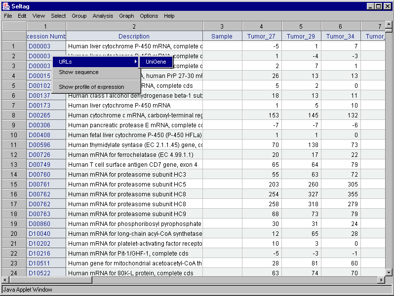
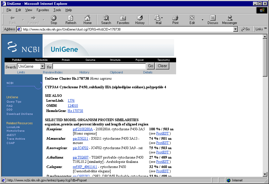
2.8. In contextual menu of the application main table (contextual menu can be called out by mouse right click) the "URLs>UniGene" command (fig. 2.8.1) will become active. This command opens you default web browser and, using the appropriate link, loads a gene card from UniGene database (fig. 2.8.2).
2.9. To load a file with genes nucleotide sequences, select the "File>Link sequence" command from the main menu (fig. 2.9).
2.10. The "Load data" dialog with files and information on their size (fig. 2.10) will appear. Select the file of interest and press "OK".
2.11. The "Description load" dialog with invitation to use dynamic file loading mode (fig. 2.11) will appear. Press the "Yes" button.
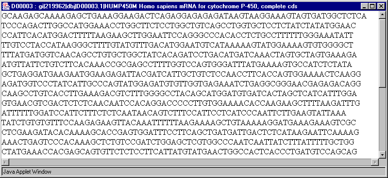
2.12. In contextual menu of the application main table (contextual menu can be called out by mouse right click) the "Show sequence" command (fig. 2.8.1) will become active. This command opens a window with gene's nucleotide sequence (fig. 2.12).
2.13. To get a description of loaded data, select the "File>Data description" command from the main menu (fig. 2.13).
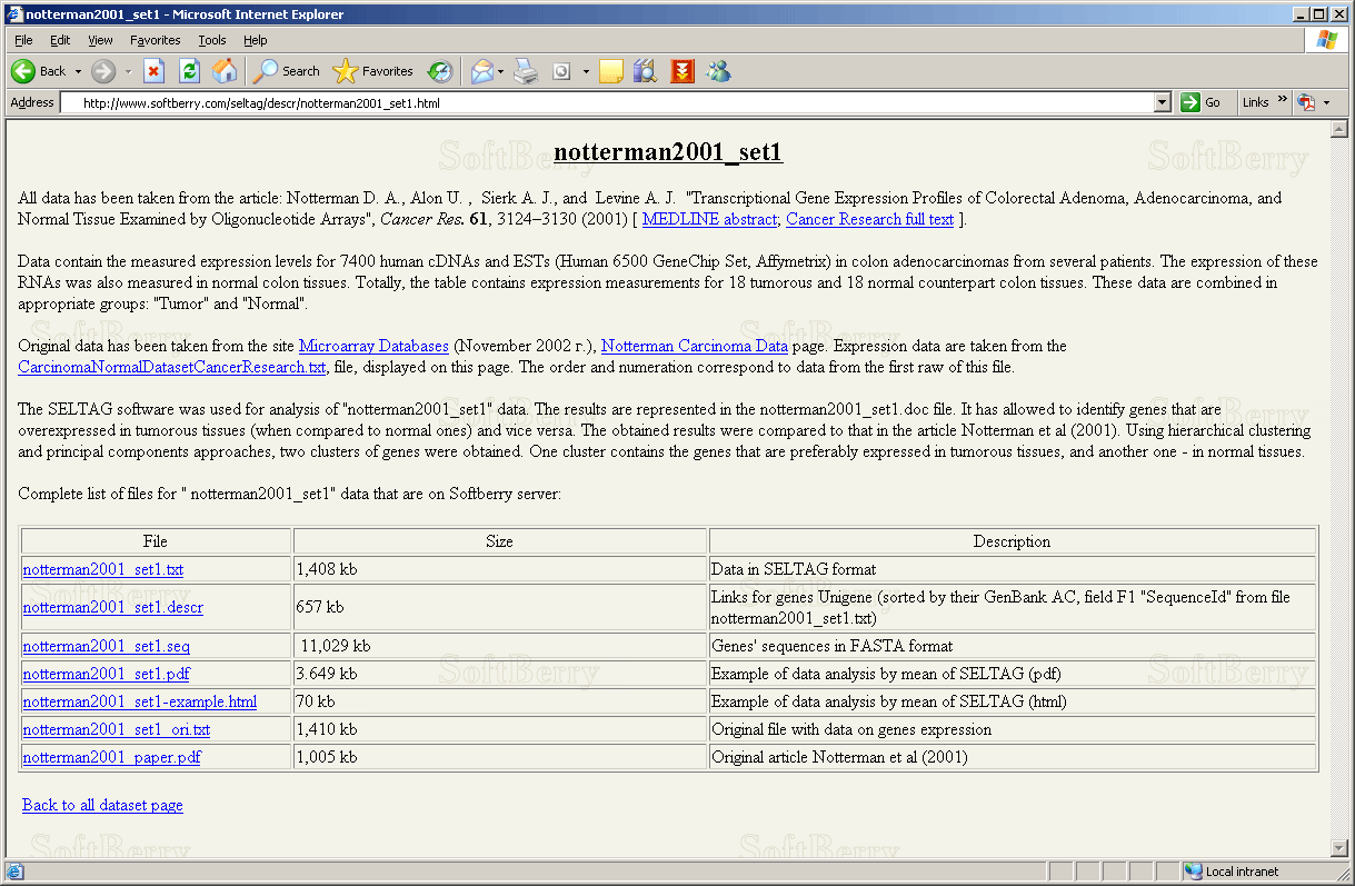
2.14. It will open the document with description and list of files for data "notterman2001_set1", located on the Softberry server (fig. 2.14).
In this chapter there is an example of how to select genes, which are expressed above average (more than 50) in, at least, 80% of tumorous tissues and, at the same time, below average (less than 50) in, at least, 80% of normal ones. The previously described dividing of experiments into two groups (in accordance with tissue types) - tumorous (G1) and normal (G2) - in the notterman2001_set1.txt file makes the solving of this task much easier.
To perform this task, the following steps are required:
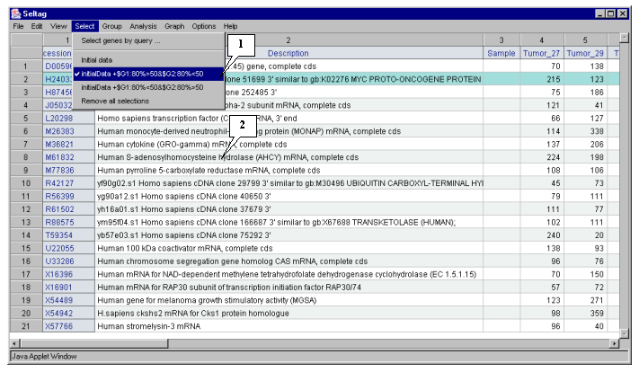
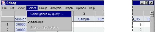
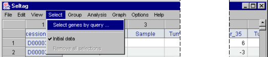
3.1. Select the "Select>Select genes by query�" command from the main menu (fig. 3.1).
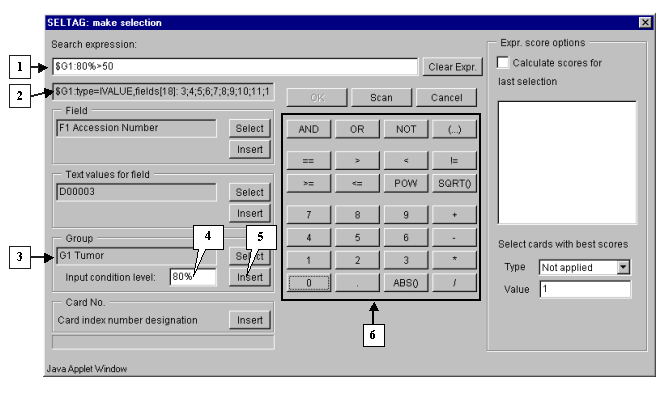
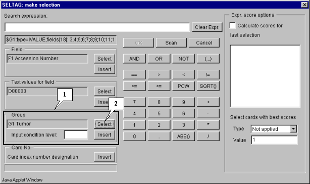
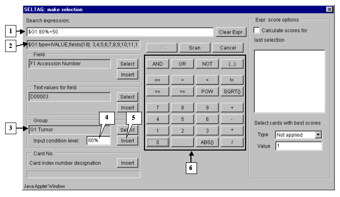
3.2. The "Make selection" dialog will appear (fig. 3.2). For the first, select a target group to satisfy selection criteria. In the "Group" section press the "Select" button (fig. 3.2).
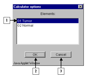
3.3. The "Calculator options" dialog with the complete list of groups in the table (fig. 3.3) will appear. In the list select a target group, for which the first part of constrains will be set. In our case, this is group "G1 Tumor". After selection press the "OK" button.
3.4. In the "Make selection" dialog the following changes will occur (fig. 3.4):
3.5.
In the field of additional constraints "Input condition level:" specify the threshold as a percentage share in a group:
80%
3.6.
The selected group ID and selection criteria should be inserted into expression line. To do this, press the "Insert" button. In the expression line the following will appear (fig. 3.4):
$G1:80%
3.7.
Using buttons of query entering specify the first part of condition in the expression line (fig. 3.4):
$G1:80%>50
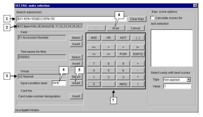
3.8. Add the "&" symbol into expression line by pressing the "And" button in the query entering section.
3.9.
Finally, specify the second part of selection criteria. It can be done by the same way, as described in 3.2-3.7, with the only exception: select the group G2 Normal and add a constraint for it:
$G2:80%<50
The final expression is shown on figure 3.5.
3.10. To start the search process press the "Scan" button (fig. 3.5). As a result, all genes, overexpressed in, at least, 80% of tumorous tissues, and downexpressed in 80% of normal ones, will be found and selected.
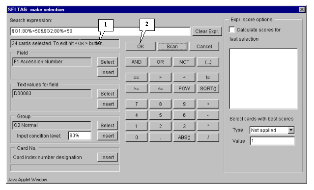
3.11. Once the selection is finished, information on the number of found genes will be represented in the status bar (fig. 3.6), and the "OK" button will become active.
3.9. Press the "OK" button.
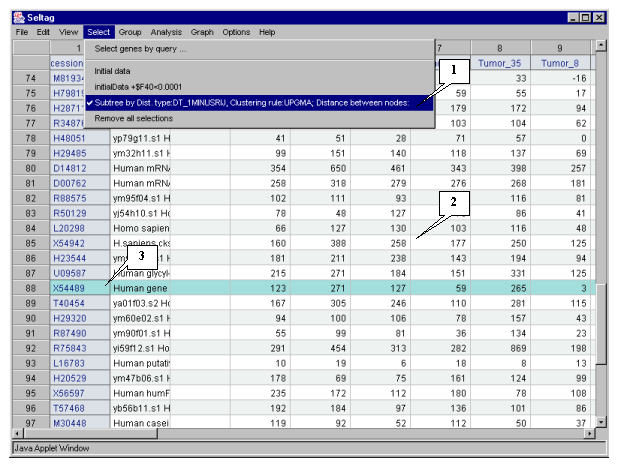
3.10. In the application main window the table with selected genes (fig. 3.7) will be represented. In the "Select" section of the main window menu an additional item with the name corresponding to selected set of genes will appear. During the project run, the obtained sets of genes can be saved and remained available by simple switching between them. To remove the list of tables use the "Remove all selections" command.
Table obtained in this example includes 21 genes. Some of selected genes are also identified as transcripts that overexpressed in tumorous tissues (when compared to their normal counterparts) in the article by Notterman et al [1] (see table 1 in this article). These genes are:
X54489 Human gene for MGSA
U22055 Human 100 kDA coactivator mRNA, complete cds
M61832 Human S-adenosylhomocysteine hydrolase (AHCY) mRNA, complete cds
M36821 Human cytokine (GRO-g) mRNA, complete cds
U33286 Human chromosome segregation gene homolog CAS mRNA, complete cds
X54942 H. sapiens CKSHS2 mRNA for CKS1 protein homologue
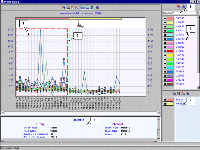
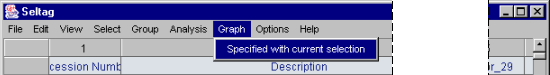
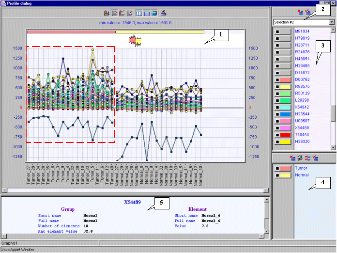
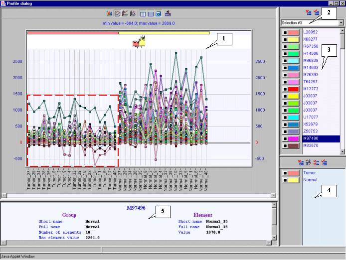
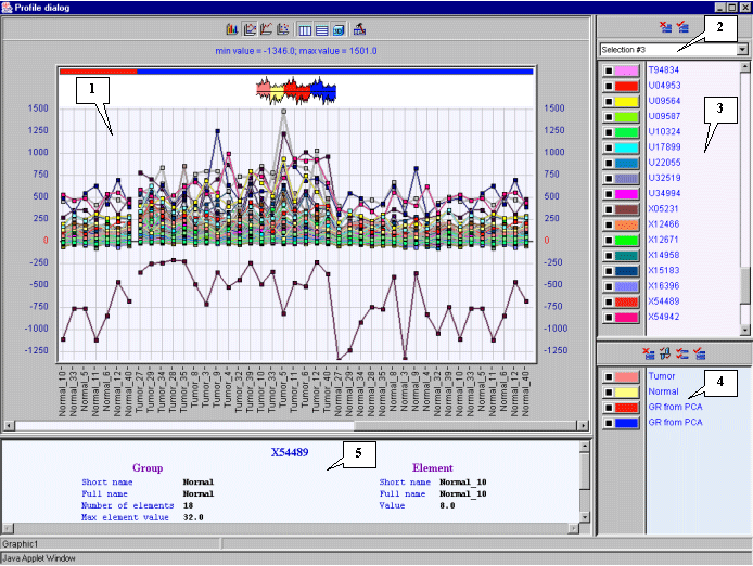
3.11. To visualize expression profiles for selected genes, use the "Graph>Specified with current selection" command from the main menu (fig. 3.8).
3.12. The "Profile dialog" window with expression profiles for selected genes (fig. 3.9) will appear. It is notable that expression profiles of all represented genes are higher for tumorous tissues (profiles inside the red rectangle) than for normal ones (profiles outside the red rectangle).
In this chapter there is an example of how to select genes, which are expressed above average (more than 50) in, at least, 80% of normal tissues and, at the same time, below average (less than 50) in, at least, 80% of tumorous ones.
To perform this task, the following steps are required:
4.1. Select the "Select>Select genes by query�" command from the main menu (fig. 4.1).
4.2. The "Make selection" dialog will appear (fig. 4.2). For the first, select a target group to satisfy selection criteria. In the "Group" section press the "Select" button (fig. 4.2).
4.3. The "Calculator options" dialog with the complete list of groups in the table (fig. 4.3) will appear. In the list select a target group, for which the first part of constrains will be set. In our case, this is group "G1 Tumor". After selection press the "OK" button.
4.4. In the "Make selection" dialog the following changes will occur (fig. 4.4):
4.5.
In the field of additional constraints "Input condition level:" specify the threshold as a percentage share in a group:
80%
4.6.
The selected group ID and selection criteria should be inserted into expression line. To do this, press the "Insert" button. In the expression line the following will appear (fig. 4.4):
$G1:80%
4.7.
Using buttons of query entering, specify the first part of condition in the expression line (fig. 4.4):
$G1:80%>50
4.8. Add the "&" symbol into expression line by pressing the "And" button in the query entering section.
4.9.
Finally, specify the second part of selection criteria. It can be done by the same way, as described in 3.2-3.7, with the only exception: select the group G2 Normal and add a constraint for it:
$G2:80%>50
The final expression is shown on figure 4.5.
4.10. To start the search process press the "Scan" button (fig. 4.5).
4.11. Once the selection is finished, information on the number of found genes will be represented in the status bar (fig. 4.6), and the "OK" button will become active.
4.12. Press the "OK" button.
4.13.
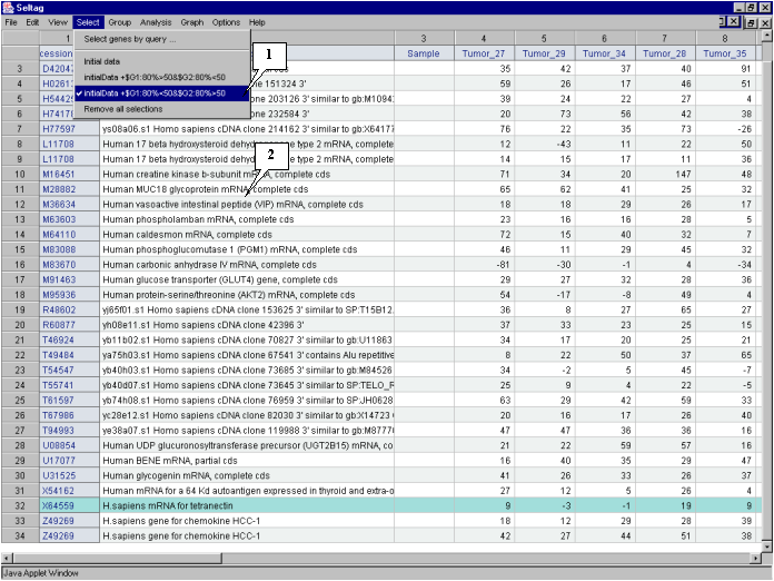
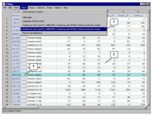
In the application main window the table with selected genes (fig. 4.7) will be represented. In the "Select" section of the main window menu an additional item with the name corresponding to selected set of genes will appear. During the project run, the obtained sets of genes can be saved and remained available by simple switching between them. To remove the list of tables use the "Remove all selections" command.
Table obtained in this example includes 34 genes. Some of selected genes are also identified as
transcripts that overexpressed in normal tissues (when compared to their tumor counterparts)
in the article by Notterman et al [1] (see table 2 in this article). These genes are:
M83670 Human carbonic anhydrase IV mRNA, complete cds
X64559 H. sapiens mRNA for tetranectin
T54547 H. sapiens cDNA similar to M84526 complement factor D precursor
M95936 Human protein-serine/threonine (AKT2) mRNA, complete cds
T46924 H. sapiens cDNA similar to gb:U11863 amiloride-sens amine oxidase
L11708 Human 17 b-hydroxysteroid dehydrogenase type 2 mRNA, complete cds
H54425 H. sapiens cDNA similar to gb:M10942_cds1 human metallothionein-le gene
H77597 H. sapiens cDNA similar to gb:X64177 H. sapiens mRNA for metallothionein
T67986 H. sapiens cDNA clone 82030 39 similar to gb:X14723 clusterin precursor
U17077 Human BENE mRNA, partial cds
U08854 Human UDP glucuronosyltransferase precursor (UGT2B15) mRNA, complete cds
4.14. To visualize expression profiles for selected genes, use the "Graph>Specified with current selection" command from the main menu (fig. 4.8).
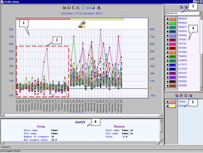
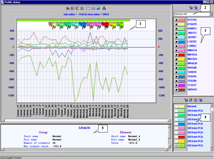
4.15. The "Profile dialog" window with expression profiles for selected genes (fig. 4.9) will appear.
It is notable that expression profiles of all represented genes are lower for tumorous tissues (profiles inside the red rectangle) than for normal ones (profiles outside the red rectangle).
From genes overexpressed in tumorous tissues we have selected the "Human gene for melanoma growth stimulatory activity (MGSA)", GenBank accession number X54489.
In current chapter it is described how to find genes having expression profiles similar to that of MGSA. As the similarity measure, the Pearson's correlation coefficient for expression profiles will be used.
To perform this task, the following steps are required:
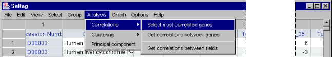
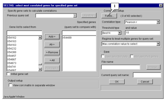
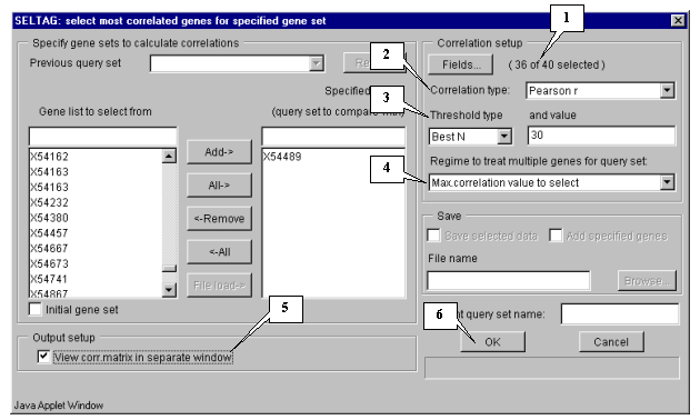
5.1. Use the "Analysis>Correlations>Select most correlated genes" command from the main menu to call the "Select most correlated genes for specified gene set" dialog (fig. 5.1).
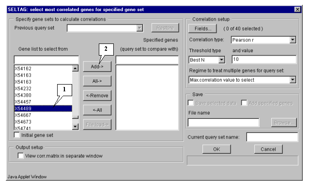
5.2. Specify the sets of genes to calculate correlations between them by selecting the appropriate gene, which will be used as the base for correlation analysis (in our case, this is gene "X54489" - MGSA), from the "Gene list to select from" list (fig. 5.2). Once gene is selected, press the "Add" button, and it will be relocated into "Specified genes" list (fig. 5.3).
5.4. Specify the calculation parameters:
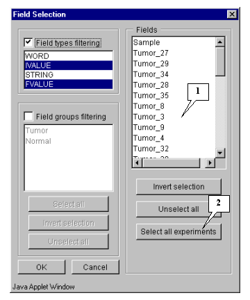
5.4.1. Specify fields that will be used for calculation by pressing the "Fields" button (fig. 5.3). The "Field selection" dialog (fig. 5.4.1.1) will appear.
In this example, calculation is based on expression measurements, i.e. all numeric fields, except "Sample" and "T-Test_tumor_vs._Normal", are used.
Press the "Select all experiments" button to select all fields, and then remove selection from the mentioned fields by clicking mouse on their names (fig. 5.4.1.2).
Press the "OK" button.
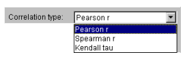
5.4.2. Select the appropriate correlation type from the "Correlation type" list (fig. 5.4.2). In this example, the Pearson's correlation coefficient is used.
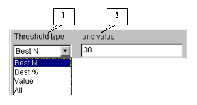
5.4.3. Choose the correlation threshold type (fig. 5.4.3). If the "Best N", "Best %" or "Value" threshold types are selected, in the "and value" field specify the threshold value. In the current example, the "Best N" type with value 30 is used. It means that after calculations 30 genes with maximal absolute values of correlation coefficients with the target gene MGSA expression profile will be selected.
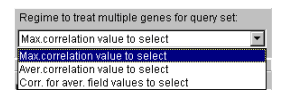
5.4.4. Choose the appropriate mode from the "Regime to treat multiple genes for query set" list (fig. 5.4.4). In this example, the "Max. correlation value to select" mode is used.
5.5. Specify the data output parameters. In this example, it is required to get a matrix with correlation coefficients in a separate window. To do this, check in the "View corr. matrix in separate window" checkbox (fig. 5.5).
Comment. The figure 5.5 represents the selected calculation parameters.
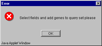
5.6. Press the "OK" button (fig. 5.5). If sets of genes are not formed or fields for calculations are not selected, the "Error" message box (fig. 5.6) will appear.
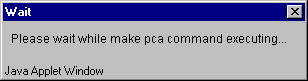
5.7. During the data processing the "Wait" message (fig. 5.7) appears, and once the process is over it disappears.
5.8. Results of data processing:
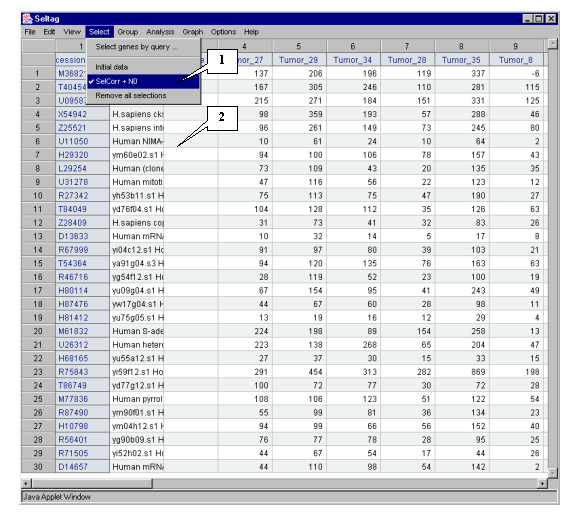
5.8.1. In the main window the table with selected genes will be represented (fig. 5.8.1). Into the "Select" menu section the new "SelCorr + N0" item corresponding to current set of genes will be added.
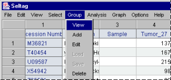
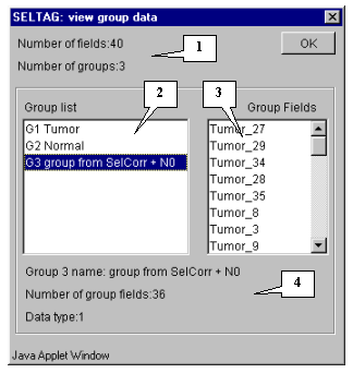
5.8.2. If to open the "View group data" dialog (using the "Group>View" command from the main menu - fig. 5.8.2.1), then one can see that in the list of experiments the new "group from SelCorr +N0" item with fields used for calculations (fig. 5.8.2.2) has appeared.
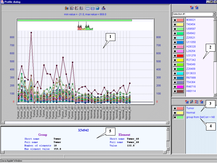
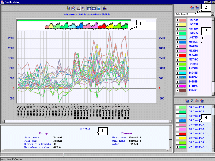
5.8.3. The "Profile dialog" window (fig. 5.8.3) with expression profiles for selected genes will appear.
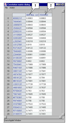
5.8.4. Since the "View corr. matrix in separate window" checkbox in the "Select most correlated genes for specified gene set" dialog was checked in, the correlation matrix's window with correlation coefficients obtained in data processing (fig. 5.8.4) will appear.
The figure 5.8.4 shows that genes with GenBank accession numbers M36821, T40454, U09587, X54942 � Z25521 have expression profiles, which correlate with that of target X54489 gene in larger degree than others.
In this chapter, the task of clustering genes by similarity of their expression profiles will be considered. For the first, genes with expression in tumorous tissues that significantly (by Student's criterion) differs from that in normal tissues (genes for which the value "T-Test_tumor_vs._normal" is lesser than 0.0001) should be selected.
To perform this task, the following steps are required:
6.1. Use the "Select>Select genes by query�" command from the main menu (fig. 6.1).
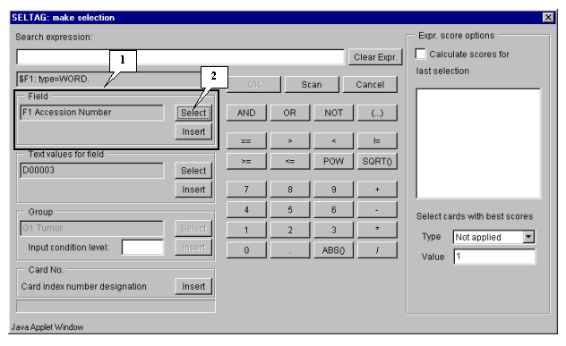
6.2. The "Make selection" dialog (fig. 6.2) will appear. For the first, choose a field, which will be used for selection. In the "Field" section press the "Select" button (fig. 6.2).
6.3.
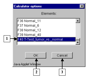
The "Calculator options" dialog with complete list of fields in the table (fig. 6.3) will appear. In the list select a field, which will be used for search. In our case it is the field:
"F40 T-Test_tumor_vs._normal".
Press the "OK" button.
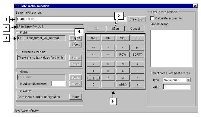
6.4. In the "Make selection" dialog the following changes will occur (fig. 6.4):
6.5.
Selected field ID should be inserted into expression line. To do this, press the "Insert" button. In the expression line the following will appear:
$F40
6.6.
Using buttons of query entering specify the condition in the expression line (fig. 6.4):
$F40<0.0001
6.7. To start the search process press the "Scan" button (fig. 6.4).
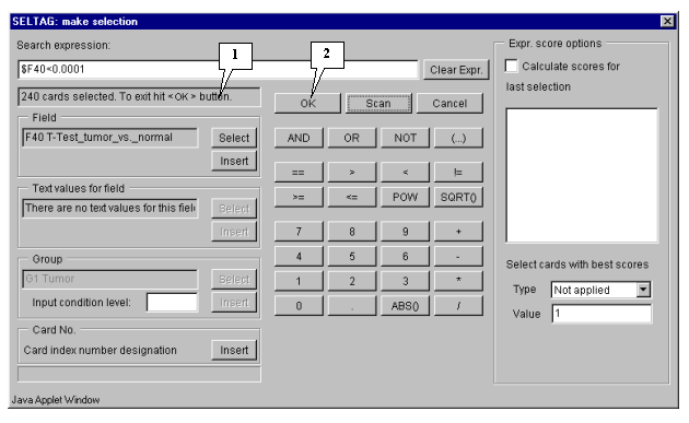
6.8. Once the selection is finished, information on the number of found genes will be represented in the status bar (fig. 6.5), and the "OK" button will become active.
6.9. Press the "OK" button.
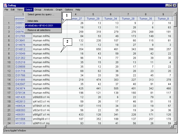
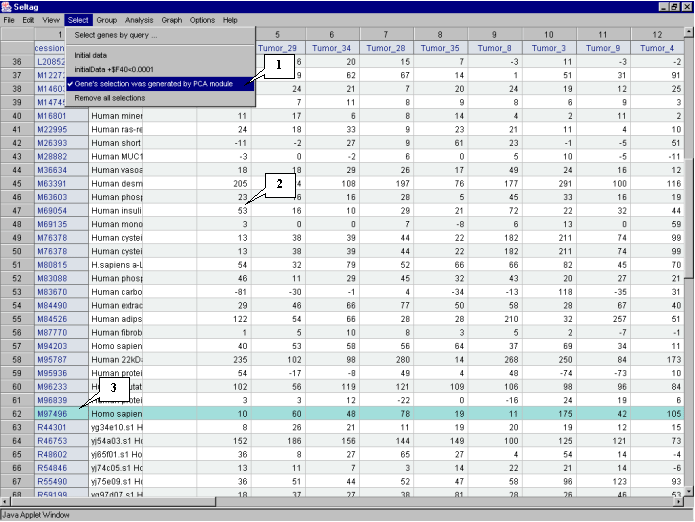
6.10. In the application main window the table with selected genes (fig. 6.6) will be represented. In the "Select" section of the main window menu an additional item with the name corresponding to selected set of genes will appear. During the project run, the obtained sets of genes can be saved and remained available by simple switching between them. To remove the list of tables use the "Remove all selections" command.
As a result, the set of 240 genes with significant differences in expression between normal and tumorous tissues have been obtained. The further analysis will be performed for this set of genes.
One of the approaches for revealing the clusters of genes with similar expression profiles is the hierarchical clustering [2]. This approach is based on building a binary tree for genes using a specified metrics of distance between their expression profiles. Each tree node binds two descending nodes and branches lengths correspond to distances between expression profiles.
To perform this task, the following steps are required:
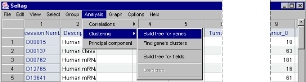
7.1. Use the "Analysis>Clustering>Build tree for genes" command from the main menu (fig. 7.1).
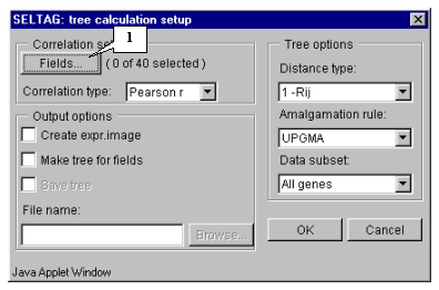
7.2. The "Tree calculation setup" dialog (fig. 7.2) will appear. For the first, choose the fields that will be used for calculations by pressing the "Fields" button.
7.3. The "Field selection" dialog (fig. 7.3) with the list of fields will appear.
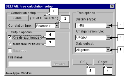
7.4. In this example, all fields, except the "Sample" and "T-Test_tumor_vs_Normal" ones, are used for calculations. Press the "Select all experiments" button (fig. 7.3) to select all fields and then remove selection from the appropriate ones ("Sample" and "T-Test_tumor_vs_Normal") (fig. 7.4).
7.5. Press the "OK" button. In the "Tree calculation setup" dialog, in the area near the "Fields" button, the information on the number of selected fields will be represented (fig. 7.5). After this, do the following:
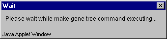
7.6. Press the "OK" button. The "Wait" message box (fig. 7.6.) will appear for the duration of calculation process.
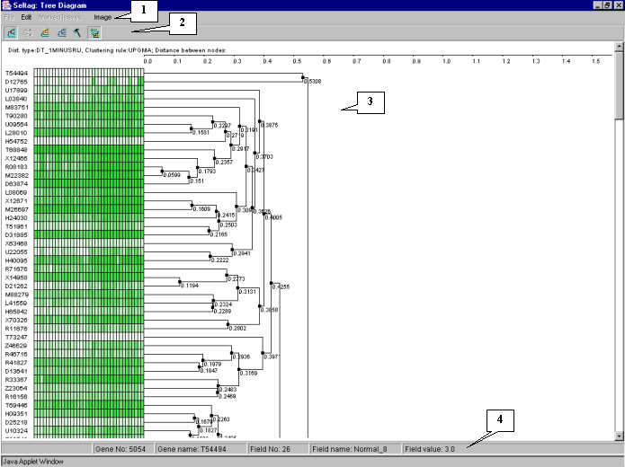
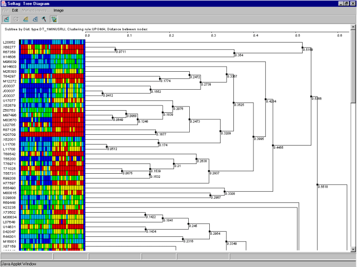
7.7. The "Tree Diagram" window with the tree of genes and expression matrix (fig. 7.7) will appear.
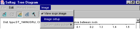
7.8. For more illustrative representation of the expression matrix, change the appropriate parameters. Use the "Image>Image setup" command from the main menu (fig. 7.8).
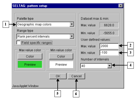
7.9. The "Pattern setup" dialog (fig. 7.9) will appear. In this window, the following settings should be changed:
7.10.
It is illustrative on the tree diagram, that genes are divided into two large clusters.
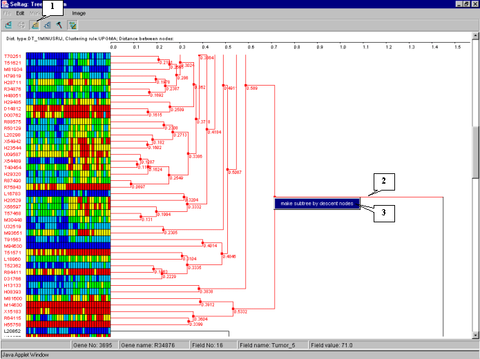
To continue analysis for the one of them only, press the ![]() button to turn on the mode for selection of descending nodes by mouse clicking, and click on the root node of the cluster. All nodes and branches of the selected cluster (cluster 1 for the further) will be highlighted by red (fig. 7.10). Click on the selected cluster by the right mouse button and choose the appeared "Make subtree by descent nodes" command (fig. 7.10).
button to turn on the mode for selection of descending nodes by mouse clicking, and click on the root node of the cluster. All nodes and branches of the selected cluster (cluster 1 for the further) will be highlighted by red (fig. 7.10). Click on the selected cluster by the right mouse button and choose the appeared "Make subtree by descent nodes" command (fig. 7.10).
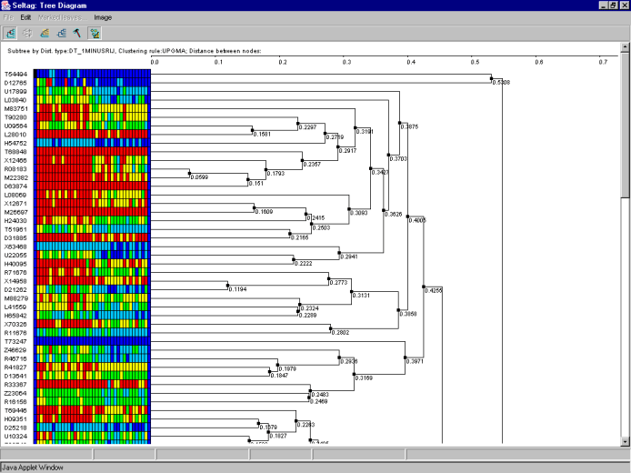
7.11. The window with tree and expression matrix for cluster 1 will appear (fig. 7.11). It is notable that color expression diagram is characterized by division of experiments (all columns except the first and the last ones) into two groups. The left part of diagram for the cluster of genes, shown on figure 7.11, has the higher expression level than the right one. In this case, the left part represents the expression values for the tumorous tissues. Such a division is a result of additional clustering of tissues simultaneously with that of genes (option 7 of panel on figure 7.5)
7.12. The table with genes from the cluster 1 (fig. 7.12) will be represented in the main window. It is illustrative that genes X54489 and X54942 with high expression in tumorous tissues have been included in this table.
7.13. In the main window choose the "Graph>Specified with current selection" command of the main menu. The "Profile Dialog" window with expression profiles of genes from the cluster 1 (fig. 7.13) will appear. It is illustrative that, for this cluster, the expression values in tumorous tissues (profiles inside the red rectangle) are higher than in normal ones (profiles outside the red rectangle).
7.14. Perform the steps described in 7.10-7.13 for the second cluster. The obtained tree, table of genes and profiles of genes for the cluster 2 are shown in the figures 7.14-7.16. It is illustrative that, for this cluster, the expression values in tumorous tissues (profiles inside the red rectangle) are lower than in normal ones (profiles outside the red rectangle) (fig. 7.16).
Thus, the hierarchical clustering analysis has allowed to select two clusters of genes that differ in their relative expression values in tumorous and normal tissues.
In the current chapter, the usage of principal components [3] in a nalysis of 240 selected genes expression is described. During the analysis, the expression table is being represented as a cloud of dots in multidimensional space. Each coordinate of this space represents the expression in appropriate tissue (experiment), and genes are represented as dots, location of which is defined by the expression values in e xperiments set. In this space, the set of axes, number of which is equal to that of experiments, and which are mutually orthogonal, is being calculated. Moreover, dispersion of dots along the first axis should be absolutely maximal, the similar dispersion along the second axis should be maximal among the remaining values, etc. These axes are referred to as components. The values of dots dispersion along these axes are characterized by sets of eigenvalues for components. Directions of these axes in the space of experiments are referred to as loadings. The first k of components that have the maximal dots dispersion are referred to as k principal components. To visualize data, most commonly use k=2, and consider the plot of dots' projection onto plane of the first two components. Such a plot allows to illustrate the location of dots in multidimensional space as well as to reveal existing clusters of genes.
To perform this task, the following steps are required:
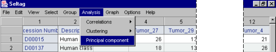
8.1. Use the "Analysis>Principal component" command from the main menu (fig. 8.1).
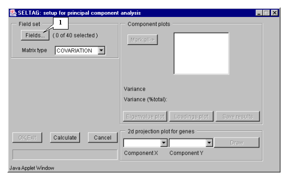
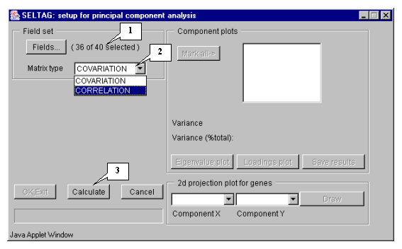
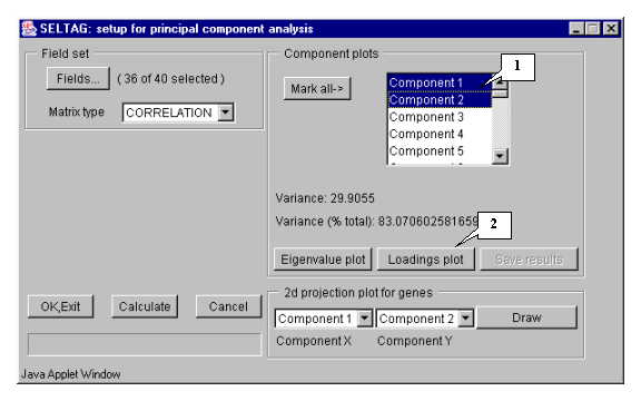
8.2. The "Setup for principal component analysis" dialog (fig. 8.2) will appear. Press the "Fields" button (fig. 8.2).
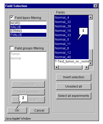
8.3. The "Field selection" dialog (fig. 8.3) that provides the choice of fields will appear.
8.4. In this example, all fields, except the "Sample" and "T-Test_tumor_vs_Normal" ones, are used for calculations. Press the "Select all experiments" button (fig. 8.3) to select all fields and then remove selection from the appropriate ones ("Sample" and "T-Test_tumor_vs_Normal") (fig. 8.4).
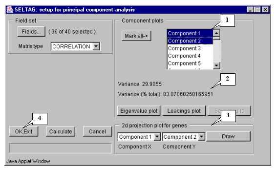
8.5. Press the "OK" button. In the "Setup for principal component analysis" dialog, in the area near the "Fields" button, the information on the number of selected fields will be represented (fig. 8.5.1). After this, do the following:
8.6. In the "Setup for principal component analysis" window, in the "Component plots" list, components (eigenvectors), numbered in descending eigenvalues order, will appear (fig. 8.6).
8.7. Choose the first and second components in the "2d projection plot for genes" section and press the "Draw" button (fig. 8.6).
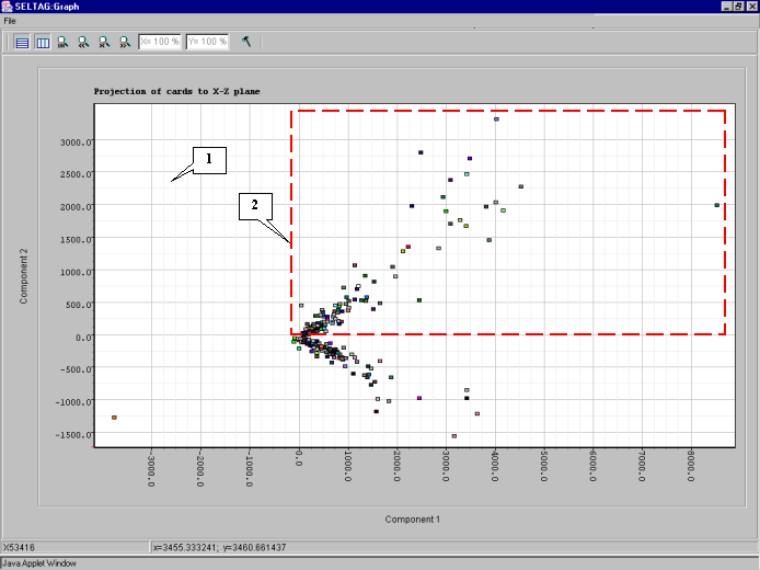
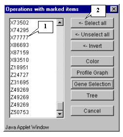
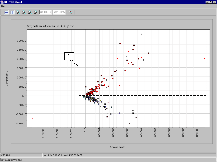
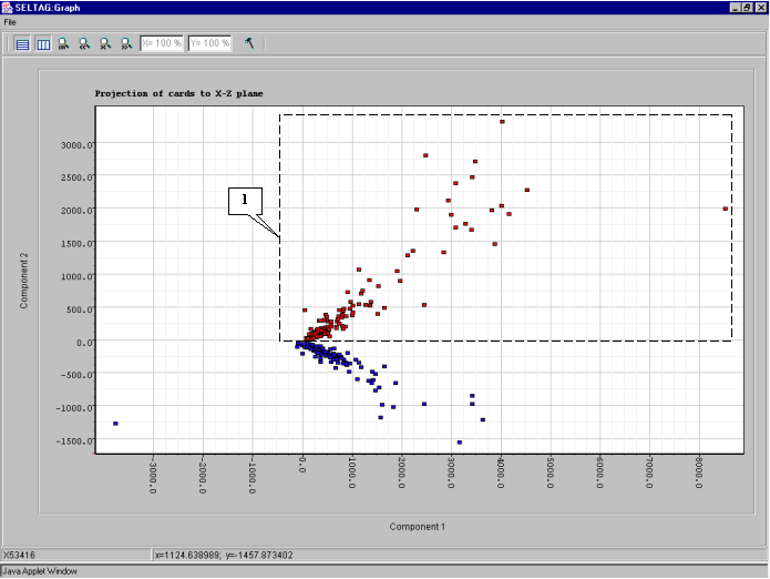
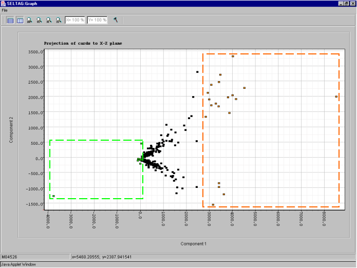
8.8. The "Graph" dialog with plot of genes distribution in the space of 2 principal components (fig. 8.8) will appear. On the plot, the two clusters along the ordinate axis can be selected. To select one of them, click the right mouse button as shown in the figure 8.8.
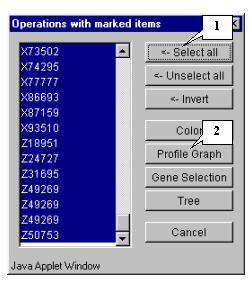
8.9. The "Operations with marked items" dialog that allows to operate the selected objects will appear. The list contains the genes of selected cluster. In order to change the color of plot objects, select all genes in the list by pressing the "<-Select all" button (fig. 8.9).
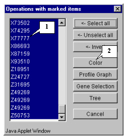
8.10. All genes in the list will become selected (fig. 8.10). Press the "Color" button.
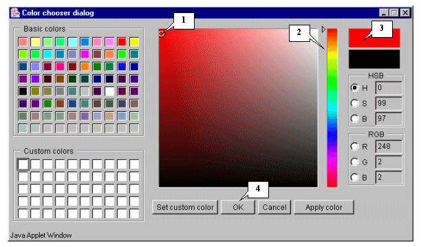
8.11. The "Color chooser dialog" window (fig. 8.11) that provides an object color selection will appear. Once selection is done, press the "OK" button.
8.12. The cluster will be painted in the selected color (fig. 8.12).
8.13. To change the color of second cluster, repeat actions 8.8-8.11. The result is shown in fig. 8.13: the red cluster will reffered to as cluster 1, and the blue one - cluster 2.
8.14. To get the diagram of cluster 1 genes' profiles, select the cluster by drawing a rectangle at hold mouse right button as shown in figure 8.13. The "Operations with marked items" dialog will appear. Select all genes by pressing the "<-Select all" button and then press the "Profile Graph" button (fig. 8.14)
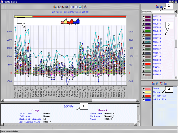
8.15. The dialog with profiles of genes in cluster 1 (fig. 8.15) will appear. It is illustrative, that genes in cluster 1 have the lower expression level in tumorous tissues than in normal ones.
8.16. In the main window, the table with genes from cluster 1 (fig. 8.16) will be represented.
8.17. On building the expression profiles for cluster 2 (blue cluster on fig. 8.13), it is illustrative that genes of this cluster are overexpressed in tumorous tissues if compared with normal ones (fig. 8.17). Thus, the second component represnts the relative expression of genes in tumorous/normal tissues. If the projection is positive, it means the gene is expressed presumably in normal tissues, if negative - in tumorous ones.
8.18. To analyse the genes distribution along the abscissa axis, i.e the first component, select the genes with minimal and maximal values of the component as shown in figure 8.18. Build the expression profiles plot (described in 8.14-8.15) for the selected genes.
8.19. Expression profiles plot for genes marked with green in figure 8.18 is shown on fig. 8.19.1. That for genes marked with orange in figure 8.18 is shown on fig. 8.19.2. When compared, it is illustrative, that genes of green cluster have the total expression level lower than that of orange one.
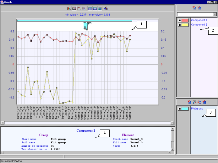
8.20. To analyze the plots for the first two components, select these components in the "Component plots" list in the "Setup for principal component analysis" dialog as shown on figure 8.20 and press the "Loadings plot" button.
8.21. The "Graph" dialog with group values for each component (fig. 8.21) will appear. It is illustrative on the plot, that all coefficients for the first component are positive and approximately equal, thus it is reasonable, that the first component is responsible for total expression level. The plot for the second component shows that for tumorous tissues all coefficients are negative, and for normal one - positive.
It is reasonable, that the first component represents total expression level in all tissues. Genes with higher projection value for this component are overexpressed, genes with projection value close to 0 are downexpressed. The second component is supposed to be responsible for expression diversities in tumors and normal tissues.
Thus, the analysis of the first two components for the set of 240 genes has allowed revealing two clusters of genes with different relative expression levels in tumors and normal tissues. At he same time, this analysis have showed that projection of expression value on the first component reflects the total gene expression level, while that on the second component characterizes relative gene expression in normal and tumorous tissues.
Represented analysis of data from the notterman2001_set1.txt file implementing several methods has allowed to select sets of genes, which are expressed differentially in normal and tumorous tissues.
1. Notterman DA, Alon U, Sierk AJ, and Levine AJ (2001) Transcriptional Gene Expression Profiles of Colorectal Adenoma, Adenocarcinoma, and Normal Tissue Examined by Oligonucleotide Arrays, Cancer Res. 61, 3124-3130.
2. Sneath P.H.A., Sokal R.R. (1973) Numerical Taxonomy. The principles and practice of numerical classification. San Francisco: W.H. Freeman and Co.
3. Everitt BS and Dunn G. Applied Multivariate Data Analysis. 1992 Oxford University Press, New York, NY.