Services Test Online
Proteomics-MSPeakFind - Softberry Mass Spectra (SMS) processing tools. Peaks identification.
On a single spectrum processing, this program performs the following operations:
(1) Data resampling;
(2) Data smoothing;
(3) Detection of the baseline and its subtraction from intensity;
(4) Normalization;
(5) Peaks identification.
Step 1. Data resampling.
The first step in mass spectra processing is data resampling. It allows to discriminate the excessive
data and to bring the mi values to common scale. As a result, different spectra will have the same
m value counts, and, thus, will be comparable. Reduction in number of spectrum points allows to lower
the noise and to eliminate excessive data, but, at the same time, to keep the spectrum shape. The common
data scale after conversion is located between the minimal and maximal m values of spectrum. The number
of data that will be resampled from original set is determined by the 'Binning percent' parameter,
that represents the percentage of spectrum points remained after conversion (default value is 25).
Example of data resampling is shown in figure 1.
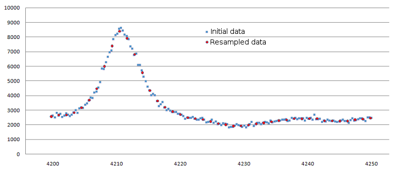
Figure 1. Result of data resampling for small spectrum interval. Original data are
shown as blue squares, resampled ones - as red circles. The 'Binning percent' for this case was set to 25.
Step 2. Smoothing.
Data smoothing procedure is intended for data noise elimination. During the smoothing, the values of
intensity for each mi point are being averaged by several neighboring points. The number
of such points is determined by the 'SmoothWindowSize' parameter (default value is 3). The smoothing
procedure can be repeated for several times; the number of iterations is determined by the 'SmoothReps'
parameter (default value is 3). Example of data smoothing is shown in the figure 2.
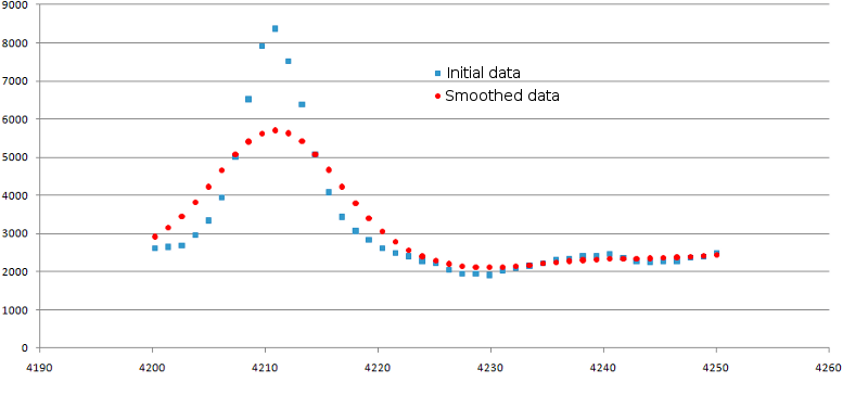
Figure 2. Result of data smoothing. Original data are shown as blue squares, smoothed ones -
as red circles. The SmoothWindowSize was set to 3 and SmoothReps was set to 3.
Step 3. Baseline detection and subtraction.
This step of data processing is applied for elimination of the systematic artifacts that occur due to matrix
and chemicals used in the experiments or as a result of detector overload. It results in background noise that
may occur to be significant for some m values. The initial step in background noise removal is
identification of peaks (local signal maxima that are located far enough from each other). The distance between
peaks is determined by the 'Baseline parameter' value (default= 0.005). This parameter defines the minimal
m distance, over which the two neighboring peaks 1 and 2 are to be located in the way, when:
|m1-m2|/m1 > 'Baseline parameter'.
After peaks identification, algorithm detects the points with signal minima located in intervals between peaks. These are the base points for calculation of background noise line. Over base points the baseline for all spectrum points is built by interpolation. In case when in some spectrum parts the value of base signal exceeds the original one, the new base points selection from neighboring ones occurs.
The values of base signal intensity are subtracted from the original one. At that, if value of original signal has occurred below zero, it is equated to zero. The result of background subtraction is shown in figure 3.
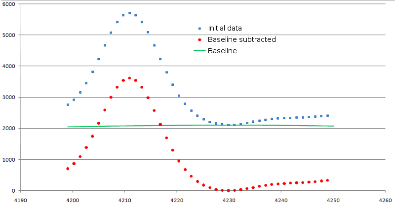
Figure 3. Result of background signal subtraction. Original data are shown as blue squares, modified ones - as red circles. Baseline is shown in green line.
Step 4. Normalization.
Normalization allows to bring peaks intensity values to a common scale, and thus it becomes possible to compare
data from different spectra. The only parameter for current procedure is 'NormalizationConstant'
(default value is 10000). Example is shown in fig. 4.
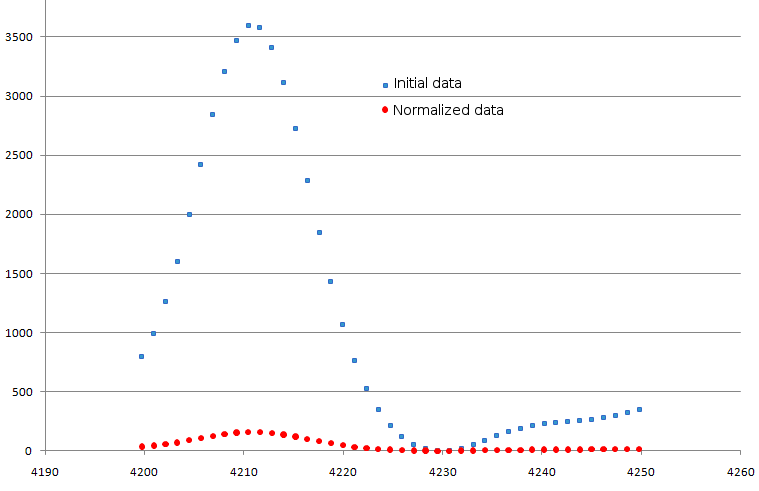
Figure 4. Result of normalization procedure. Original data are shown as blue squares, modified ones - as red circles.
Step 5. Peaks identification.
The current step of analysis lies in searching for peaks in spectrum with high signal-noise relation.
Peaks, in themselves, are identified as points of local spectrum maximum. The 'SNRMin' parameter
specifies the minimally allowed value for signal-noise relation (default value is 3). This relation is
considered in spectrum window w, size of which can be specified by the 'SNRWindowSize' parameter
(default value is 250). Thus, the value for signal-noise relation is calculated as:
![]()
Program identify peaks with SNR>'SNRMin' and intensity not less than 'MinIntensity' (default value is 2). The result is shown in fig. 5.
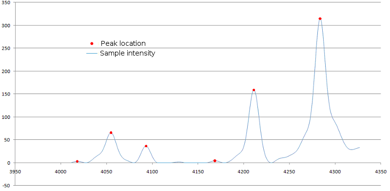
Figure 5. Identification of peaks in mass spectrum. Peaks locations over signal
curve are marked with red dots.
Input: m/z - Intensity data
Output: List of peaks with the following information for each peak:
PeakIndex (Peak ID), SampleIndex (Index of sample, for this program is always 0), PointNum
(number of point corresponding to peak location in the sample), MZRatio (m/z value), SNRRatio
(signal to noise ratio), Intensity (signal intensity).
Parameter(s):
Binning percent - This parameter specify the fraction of data in percent that will remain after resampling. The default value is 25.
SmoothWindowSize - This parameter determine window size for smoothing operation. The default value is 3.
SmoothReps - This parameter specify the number of smoothing operation repeats. The default value is 3.
Baseline parameter - This parameter specify the minimal mass difference, over which the two neighboring
peaks 1 and 2 are to be distinguished for baseline determination. The default value is 0.005.
NormalizationConstant - This parameter specify the normalization constant. The default value is 10000.
SNRWindowSize - This parameter specify window size to determine signal-to-noise ratio. The default value is 250.
SNRMin - This parameter specify minimal signal-to-noise ratio for peak detection. The default value is 3.
MinIntensity - This parameter specify minimal intensity for peak detection. The default value is 2.
File format type - This parameter specify file format. SSV-space separated values, CSV - comma separated values, TSV - tab separated values.
Data format.
Mass spectra data represent the sets of following pairs of values: mass to charge relation
(m/z, further, for more convenience, it will be referred to as m, mass) and corresponding signal intensity (I).
On a spectrum plot, the mass corresponds to X coordinate, and signal intensity- to Y one.
A typical spectrum consists of several thousand of such value pairs (points). Data are represented as
text files, where for each pair (mi,Ii) of mass-intensity values the string is assigned, and data in
this string are separated by special separator symbol. The SMS package allows several separators types:
space (SSV, space separated values, file format), comma (CSV, comma separated values, file format) and
tabulation (TSV, tab-separated values, file format). In files with data, the string with comments are
allowed; during the file reading these strings are to be skipped. The commentary strings should begin
with "#" symbol at the first position. In the figure 2 the example of file with data in CSV format is shown.
#M/Z,Intensity
-7.8602611e-005,4.1126194
2.1773576e-007,4.0764203
9.6021472e-005,4.0040221
0.00036601382,4.1186526
0.00081019477,4.0040221
0.0014285643,3.9617898
....
19742.941,4.077895
19745.564,4.0772248
19748.187,4.0772248
Figure 6. Example file with mass spectra data in CSV format.